


Contents
Scroll to:
https://doi.org/10.17747/2618-947X-2022-1-37-42
Scroll to:
Сельское хозяйство всегда было рискованным занятием, и это усугубляется постоянно меняющимися и непредсказуемыми погодными условиями. В результате климатических изменений мелкие фермеры подвергаются риску отсутствия продовольственной безопасности и высокого уровня нужды из‑за недоступности дорогостоящего сельскохозяйственного страхования. Чтобы защитить фермеров от этих рисков, были разработаны контракты индексного страхования, которые обеспечивают страхование фермера в случае недостатка или избытка осадков, так как реализация любого из этих двух сценариев ставит под угрозу ожидаемый урожай кукурузы. Стоимость индексного страхования урожайности кукурузы была рассчитана с использованием модели Блэка – Шоулза, поскольку контракт напоминает опцион «деньги или ничего». Страховые премии сравнивались при различных уровнях триггера, чтобы определить влияние изменений уровней триггера на цену контракта.
Mazviona B.W. INFLUENCE OF THE TRIGGER LEVELS IN PRICING OF THE MAIZE INDEX INSURANCE IN ZIMBABWE. Strategic decisions and risk management. 2022;13(1):37-42. https://doi.org/10.17747/2618-947X-2022-1-37-42
The uncertainty in the weather conditions has left farmers exposed to several production risks. The World Bank indicated that these risks are specific to mainly local agriculture production and socioeconomic development [Weather index insurance.., 2011]. Zimbabwe experienced floods, droughts and extreme temperatures, which in turn has reduced the agriculture production. Majority of the population in the country gets its income from agricultural activities, however this income has recently become very volatile due to the randomness of rainfall. 90% of variation in the crop production level is deeply rooted in the variation of rainfall roughly impacted by global change patterns. M.R. Carter and R.S. Janzen [Carter, Janzen, 2012] found that droughts affect the largest group of farmers and cause the highest damage costs. As a result, the contribution of agriculture to the GDP of Zimbabwe has been compromised.
In response to these net results of natural risks, the government has introduced ad hoc food aid programs. This initiative has however faced several challenges. Firstly, inadequate distribution of infrastructure as some of the recipients of these aids are usually asked to pay for transportation of the aid to their locations which is a burden to the already poverty-stricken population who cannot afford to meet these expenses resulting in them being unable to receive the aid. Secondly, these aid programs are vulnerable to mismanagement in the form of political abuse resulting in inequitable benefit distribution.
Despite these challenges, the programs have only met the one side of the net results of risks, it attempted to solve the food insecurity of the population but pretermitting that farmers farm also for income that covers the other needs of the family such as school fees and clothing amongst others. Exposure to chronic poverty is not addressed by these programs. Above all, these programs have created a culture of dependency which is a slow poison to the well-being of households and the economy of the country at large as agriculture contributed 12.8% of the country’s GDP in 2018 according to The Global Economy1.
To address the small scale farmers’ exposure to food insecurity and vulnerability to chronic poverty, there is a need for access to affordable agricultural insurance, this access will encourage farmers to use scarce resources efficiently and reduce the dependence on inadequate food aid programs. The introduction of index insurance products has been considered handy in protecting the farmers from these adverse effects of weather changes. The indemnity of these contracts depends on the trigger levels that appear at the onset of the contract as well as the estimation of the premiums of the index insurance. Therefore, there is need to assess the effect of the changes of the trigger levels in the premium estimation, hence this article focuses mainly on this evaluation.
In an attempt to respond to this challenge and fill void insurance insurers, agricultural economists, and researchers have developed an interest in the development of other insurance vehicles that will meet the needs of the small-scale farmers and benefit both parties of the contract. Such vehicles are the index insurance contracts, where the farmer is indemnified contingent on the performance of a variable or index, unlike the formal insurance contracts that pay indemnity based on the individual specific outcomes.
There are several indices which are correlated to the farm losses, that can be used to design index insurance contracts. These include rainfall, temperature, NDVI, and El Nino-Southern Oscillation indices amongst others, this ideology is supported by the International Fund for Agricultural Development [Weather index-based insurance.., 2011] who highlights that index insurance functions more effectively if there exists a strong correlation between insured losses and the selected index. Index insurance principles address the challenges that are faced by formal insurance in many ways. First, the value of the index cannot be influenced by the farmers, and the insurer therefore effectively frees of moral hazard and adverse selection respectively. It is cost-effective as it does not require field loss assessments and on-farm inspections like formal insurance. It however has some limitations. The greatest limitation is that it does not cover idiosyncratic losses such as those resulting from fire or conflicts.
According to [Hazell et al., 2010], index-based insurance is a financial product that indemnifies the farmer when pre-specified conditions of an aggregate index, or indicator are triggered.
According to [Clarke et al., 2012] triggers are developed using historical and current data and also monitored at weather stations that are closer to the insured farmer. The trigger values are selected for weather indices. The indemnity from the insurance contracts commence at these trigger values [Jensen N., Barrett C, 2016]. T.J. Lybbert and M.R. Carter calibrated rainfall index insurance with different trigger values using the percentiles of the rainfall data [Lybbert, Carter, 2014]. The contract payout is triggered for all farmers who bought the contract when the cumulative seasonal rainfall data received is above the trigger levels or below another trigger level.
[Okine, 2014; Filiapuspa et al., 2019] concluded that the price of the crop index insurance increases with an increase in trigger levels for contracts that cover shortage of rainfall. [Filiapuspa et al., 2019] found that the lowest trigger level (25th percentile) resulted in the cheapest premium (IDR 680,318.305 /ha/season), and the use of the highest percentile resulted in the most expensive premium (IDR 3,096,600.871/ha/season) and hence concluded that the premiums for rainfall index insurance covering rice farmers in the case of drought increase with increase in trigger levels. [Okine, 2014] observed that an increase in the trigger level from10.13 mm to 13.45 mm resulted in a 789.5% increase in premiums and that an increase in the trigger level from 13.45 mm to 19.42 mm produced 789.5% increase in premiums. [Kath et al., 2018] found that the cheapest premiums ($ 12.06 AUD/ha) for the excess rainfall index insurance for sugar cane was at the highest trigger level (95th percentile) and the most expensive premium($ 57.25AUD/ha) was at the lowest trigger level applied (70th percentile).
The maize yields and rainfall data used were obtained from AGRITEX and NASA website respectively. The data used for the study range from October 2009 to May 2019 for rainfall data and 2010 to 2019 for the maize yields data. The black-Scholes option pricing framework was used to evaluate the contract in the study. Normalized yields and seasonal rainfall data for the region were used in the premium estimation process. Regional data were obtained from averaging the data for the districts in the corresponding regions. The prices were estimated at different trigger levels. The changes in the estimated premiums were then computed and conclusions were made.
This section summarises the descriptive statistics (means, standard deviation, minimum and maximum) of the data used in the research. According to [Mushore, 2013] the Zimbabwean rainfall season ranges from mid of November to mid of March of the following year, therefore the cumulative seasonal rainfall in this study was taken as the cumulative rainfall for the period from the beginning of October to the beginning of May to account for the late planted crops contradicting with [Mushore et al., 2017] whose period ranged from the 1st of October to the 31st of March of the next year. The seasonal descriptive statistics for the respective regions during the period 2010-2019 are summarised in the table 1.
The average rainfall received in region I, IIA, IIB, III, IV and V is 701.39 mm, 759.96 mm, 743.45 mm, 660.02 mm, 468.25 mm and 324.95 mm respectively. The average rainfall generally decreases across the regions.
The graph below shows the trend between the maize yields and time. A downward trend is observed for all regions thus justifying the need for index insurance to cover the smallholder farmers in the event of either shortage or excess of rainfall, which occurrence leads to reduced yields.
3.1. Analysis of relationship between maize yield and seasonal rainfall
The relationship between the maize yields and rainfall was examined with the use of different regression models that include linear, log linear and quadratic schemes. The maize yields data were detrended and normalized to remove the effects of heteroskedasticity and time trends when using model 1 and 2. The normalized maize data are presented in the appendix. To test the relationship between the variables the original seasonal data were used in the case of independent variable and normalized maize yields were used in the place of dependent variable. The correlation coefficients R2 were compared. The results from the regression models analysis are summarized in the table 2.
The relationships between maize yields and rainfall were modelled better using the quadratic regression model (for all regions) compared to linear regression and nonlinear regression for the region I, IIA, IIB, III, IV, V respectively. This is indicated by the highest R2 values of 0.01, 0.07, 0.22, 0.03, 0.26 and 0.01 for regions I, IIA, IIB, III, IV and V respectively being obtained from the quadratic regression model; This showed that the maize yields increase with rainfall to a limit point where it start to decrease with excessive rainfall. Beyond this point, the maize yields begin to decrease, hence the need for index insurance will cover both drought and floods. This is similar to the findings of [Mushore et al., 2017], who concluded that the relationship between maize yields and rainfall in Mt Darwin is better modelled by a quadratic regression model with R2=0.630. The figures in this research differ from the findings as the study sampled different districts but however they both exhibit similar relationships between the variables. These findings are also in contradiction with those of [Poudel et al., 2016] who found that the crop yields were linearly related to the rainfall data. This is due to the difference in the crop type examined and the sample population.
3.2. Premium Rate estimation
Determination of trigger values
The trigger levels for drought coverage were the lower percentiles i.e. (10th, 25th, and 50th percentiles) whereas the upper percentiles i.e. (60th, 75th, and 90th percentiles) were used as the trigger levels of the floods coverage. Therefore, the trigger values for the contract will be (10th and 60th), (25th and 75th) and (50th and 90th). The percentiles for each region are summarized in table 3.
Lognormal test of seasonal rainfall data
When pricing the options using the Black-Scholes framework, it is assumed that  follows a lognormal distribution. Hence, examine if
  follows a lognormal distribution. Q-Q plots for the rainfall data were plotted to indicate that the data follow a lognormal distribution, the plots are presented in the appendix. To further prove that the data follow a lognormal distribution, Kolmogorov-Smirnov Test and Shapiro-Wilk Tests were carried out using SPSS.
H0 = the ln (seasonal rainfall) follows Normal distribution.
H1 = the ln (seasonal rainfall) does not follow Normal distribution.
The p- values of the both the Kolmogorov test and Shapiro - Wilk test are both greater than 0.05, therefore we conclude that the natural logarithm of the seasonal rainfall data with maize follows a normal distribution, hence the data follow a lognormal distribution, therefore, we accept Ho. The results of these tests are presented in the table 4.
The scatter plots below show that the log of seasonal rainfall data follows a normal distribution and hence the seasonal rainfall data follow a lognormal distribution. This similar to [Okine, 2014] findings.
Pricing
In this case, we consider a contract that pays out indemnity at a rate of 1 in the event of either drought or floods. Therefore:
Pay-out = Pay-out rate x the insured amount of yields x the preagreed value of 1 unit of maize yields.
The contract resembles an exotic combination option which consist of a cash or nothing put option struck at the lower percentiles and a cash or nothing call option struck at the upper percentiles. Therefore, the premiums paid by the insured will be the total of the premiums paid if the farmer was to purchase these options separately (drought and floods insurance separately).
Premiums = Premium of long cash or nothing put option + premium of a long cash or nothing call option
The premiums paid by a farmer from region 3 are calculated as follows:
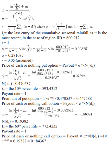
Overall premium = Price of cash or nothing put option + Price of cash or nothing call option = 0.447588 + 0.184367 = 0.631955.
There premium rate paid for both drought and floods cover is 0.631955 for a payout rate of 1 in the event of either floods or drought.
Effects of trigger levels of premium price
The premium rates for other regions at different trigger levels, i.e. percentiles are summarised in table 5. From this table it can be deduced that for region 3 the premiums increase with an increase in trigger value, hence highlighting the importance of trigger values when pricing the contract. The premium for the drought cover increased by 30.34% when the trigger increased from 493.084 mm (10th percentile) to 580.734 mm (25th percentile). When the trigger increased from 693.067 mm (60th percentile) to 752.37 mm (75th percentile), the premium rate for the floods scenario cover decreased by 62.98%. The overall premium increased by 20.89%. The percentage changes of premiums as the trigger values increase are summarized in table 6.
We concluded that, on average, when the trigger value for the drought cover is increased the price of the contract also increases as the probability of rainfall being lower than the trigger value increases hence the higher chances of loss materialization to the insurance company. This conclusion is also similar to that made by [Filiapuspa et al., 2019] who found out that the price of drought index insurance increases with trigger levels. The cost of floods insurance cover decreases with increase in the trigger levels of the contract. This is due to the decrease in the probability of the payment triggered by the lower expectation of costs.
Table 1
Regional descriptive statistics
|
Region |
Mean |
Median |
Standard Deviation |
Sample Variance |
Minimum |
Maximum |
|
|
I |
Seasonal Rainfall |
701.389 |
656.706 |
139.733 |
19525.398 |
483.984 |
971.904 |
|
Maize Yields |
0.528 |
0.559 |
0.144 |
0.021 |
0.249 |
0.709 |
|
|
IIA |
Seasonal Rainfall |
759.959 |
816.996 |
129.910 |
16876.645 |
556.884 |
924.360 |
|
Maize Yields |
0.532 |
0.508 |
0.182 |
0.033 |
0.328 |
0.829 |
|
|
IIB |
Seasonal Rainfall |
743.446 |
756.750 |
128.616 |
16542.184 |
526.104 |
996.252 |
|
Maize Yields |
0.363 |
0.365 |
0.106 |
0.011 |
0.217 |
0.535 |
|
|
III |
Seasonal Rainfall |
660.025 |
683.316 |
129.782 |
16843.320 |
441.924 |
828.456 |
|
Maize Yields |
0.312 |
0.309 |
0.085 |
0.007 |
0.205 |
0.471 |
|
|
IV |
Seasonal Rainfall |
468.251 |
447.216 |
121.503 |
14762.917 |
308.592 |
675.000 |
|
Maize Yields |
0.169 |
0.143 |
0.056 |
0.003 |
0.117 |
0.272 |
|
|
V |
Seasonal Rainfall |
324.954 |
587.700 |
105.583 |
11147.836 |
504.564 |
835.620 |
|
Maize Yields |
0.214 |
0.173 |
0.075 |
0.006 |
0.146 |
0.347 |
Fig. 1. Maize Yields
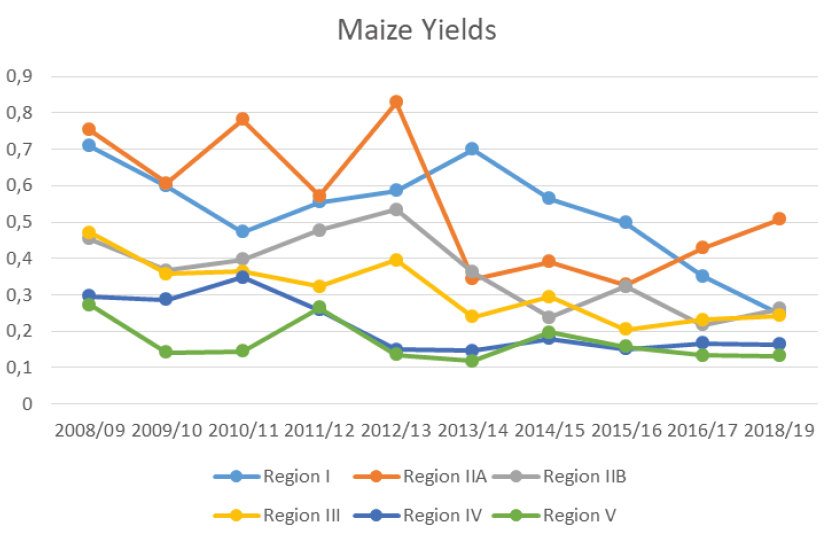
Table 2
Regression model results
|
Region |
I |
IIA |
IIB |
III |
IV |
V |
|
|
Linear model |
R2 |
0.00 |
0.05 |
0.18 |
0.02 |
0.16 |
0.00 |
|
Intercept |
717.90 |
841.66 |
484.46 |
783.43 |
789.95 |
461.61 |
|
|
X Coefficient |
-24.40 |
-127.90 |
597.30 |
-266.64 |
-580.07 |
26.12 |
|
|
Log Linear model |
R2 |
0.00 |
0.03 |
0.20 |
0.02 |
0.13 |
0.00 |
|
Intercept |
691.14 |
725.42 |
966.87 |
563.94 |
461.15 |
474.36 |
|
|
X Coefficient |
-24.29 |
-65.60 |
260.67 |
-122.93 |
-126.70 |
4.33 |
|
|
Quadratic model |
R2 |
0.01 |
0.07 |
0.22 |
0.03 |
0.26 |
0.01 |
|
Intercept |
857.25 |
630.15 |
-5.18 |
1452.05 |
362.08 |
688.91 |
|
|
X Coefficient |
-505.03 |
559.39 |
2965.48 |
-3285.75 |
3036.82 |
-1939.94 |
|
|
X2 coefficient |
385.66 |
-508.46 |
-2745.61 |
3330.90 |
-7022.84 |
3908.56 |
Table 3
Trigger levels (percentiles)
|
Percentile |
Region I |
Region IIA |
Region IIB |
Region III |
Region IV |
Region V |
|
10th |
594.770 |
644.753 |
593.431 |
493.084 |
518.885 |
334.415 |
|
25th |
621.459 |
680.625 |
687.630 |
580.734 |
558.972 |
380.112 |
|
50th |
656.706 |
786.940 |
756.750 |
683.316 |
587.700 |
447.216 |
|
60th |
690.022 |
818.359 |
772.423 |
693.067 |
630.934 |
470.345 |
|
75th |
767.382 |
858.510 |
796.482 |
752.370 |
690.402 |
569.811 |
|
90th |
869.876 |
879.518 |
839.533 |
816.360 |
741.217 |
605.351 |
Source: author’s analysis.
Table 4
Normality test results
|
Kolmogorov - Smirnova |
Shapiro - Wilk |
|||||
|
Statistic |
df |
Sig. |
Statistic |
df |
Sig. |
|
|
Region 1 |
0.196 |
10 |
0.200b |
0.967 |
10 |
0.864 |
|
Region 2A |
0.214 |
10 |
0.200b |
0.932 |
10 |
0.465 |
|
Region 2B |
0.167 |
10 |
0.200b |
0.961 |
10 |
0.796 |
|
Region 3 |
0.198 |
10 |
0.200b |
0.936 |
10 |
0.513 |
|
Region 4 |
0.196 |
10 |
0.200b |
0.941 |
10 |
0.561 |
|
Region 5 |
0.152 |
10 |
0.200b |
0.965 |
10 |
0.836 |
a Lilliefors significance correction.
b This is a lower bound of the true significance.
Fig. 2. Normal Q-Q plot of Regions
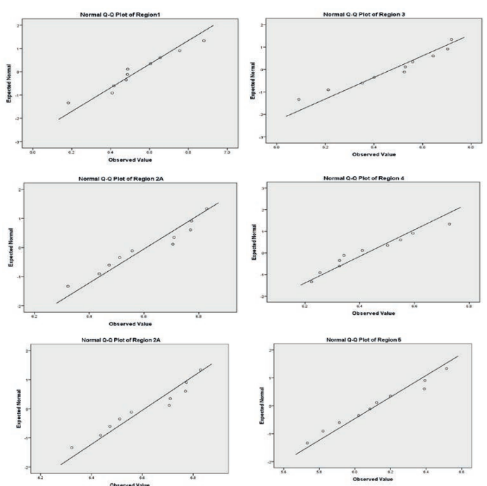
Table 5
Estimated Premiums
|
Trigger |
Region I |
Region IIA |
Region IIB |
Region III |
Region IV |
Region V |
|
|
Premiums of drought cover (1) |
10th |
0.1946 |
0.2195 |
0.4476 |
0.4651 |
0.5365 |
0.5705 |
|
25th |
0.2347 |
0.3022 |
0.6409 |
0.6677 |
0.6490 |
0.7015 |
|
|
50th |
0.2906 |
0.5618 |
0.7472 |
0.8189 |
0.7166 |
0.8266 |
|
|
Premiums of floods cover (2) |
60th |
0.6059 |
0.3212 |
0.1844 |
0.1224 |
0.1547 |
0.0967 |
|
75th |
0.4796 |
0.2450 |
0.1572 |
0.0751 |
0.0823 |
0.0309 |
|
|
90th |
0.3311 |
0.2105 |
0.1170 |
0.0433 |
0.0459 |
0.0203 |
|
|
Overall premiums (1+2) |
10th and 60th |
0.8005 |
0.5407 |
0.6320 |
0.5876 |
0.6911 |
0.6672 |
|
25th and 75th |
0.7143 |
0.5472 |
0.7981 |
0.7428 |
0.7313 |
0.7324 |
|
|
50th and 90th |
0.6218 |
0.7723 |
0.8642 |
0.8621 |
0.7625 |
0.8469 |
Source: аuthor’s analysis.
Table 6
Changes in the premium rates
|
Trigger |
Region I |
Region IIA |
Region IIB |
Region III |
Region IV |
Region V |
|
|
Premiums of drought cover((1) |
10th |
- |
- |
- |
- |
- |
- |
|
25th |
17.062 |
27.376 |
30.159 |
30.335 |
17.345 |
18.677 |
|
|
50th |
19.261 |
46.204 |
14.232 |
18.464 |
9.429 |
15.134 |
|
|
Premiums of floods cover(2) |
60th |
- |
- |
- |
- |
- |
- |
|
75th |
-26.330 |
-31.104 |
-17.274 |
-63.056 |
-88.047 |
-213.125 |
|
|
90th |
-44.830 |
-16.417 |
-34.407 |
-73.580 |
-79.059 |
-52.061 |
|
|
Overall premiums (1+2) |
- |
- |
- |
- |
- |
- |
|
|
-12.074 |
1.194 |
20.815 |
20.894 |
5.490 |
8.906 |
||
|
-14.872 |
29.139 |
7.649 |
13.845 |
4.098 |
13.523 |
Source: аuthor’s analysis.
It was found out that the overall premium rates increased with the increase in trigger levels for the contract. The contract is a combination of drought and floods insurance cover. It was noted that the price of the drought cover separately grew with an increase in trigger levels as the probability of occurrence of the insured event increased. The price of the floods cover was decreasing with the increase in the trigger levels as the probability of the payments being triggered reduced since a majority of the rainfall entries from the collected data were much below these triggers. The overall premium of the contract that covers both droughts and floods generally increased with an increase in trigger levels. This was due to the higher probability of droughts occurence compared to that of floods. It was also found that the price of the contract increased with the increase in the trigger levels of the contract. This was in line with the observations of Okine (2014) who noted that the price of the drought insurance increased with the increase in trigger levels. The price of the contact varied linearly with the price of the drought cover and inversely with the price of the floods cover if these were purchased separately. This was found to be due to the lower likelihood of floods occurrence, which was overpowered by the likelihood of droughts in the period considered in this research.
1 The Global Economy - 2018: https://reports.weforum.org/global-competitiveness-report-2018/country-economy-profiles/.
1. Carter M.R., Janzen R.S. (2012). Coping with drought: Assessing the impacts of livestock insurance in Kenya. I4 Brief No. 2012-1, University of California - Davis, Index Insurance Innovation Initiative, Davis, CA.
2. Clarke M., Lodge A., Shevlin M. (2012). Evaluating initial teacher education programmes: Perspectives from the Republic of Ireland. Teaching and Teacher Education, 28: 141-153.
3. Hazell P., Anderson J., Balzer N., Clemmensen H., Hess U., Rispoli F. (2010). The potential for scale and sustainability in weather index insurance for agriculture and rural livelihoods. Rome.
4. Lybbert T.J., Carter M.R. (2014). Bundling drought tolerance and index insurance to reduce household vulnerability to drought. Sustainable Economic Development: Resources, Environment, and Insitutions, Elsevier Inc.: 401-414. https://doi.org/10.1016/B978-0-12- 800347-3.00022-4.
5. Jensen N., Barrett C. (2016). Agricultural index insurance for development. Applied Economic Perspectives and Policy, 39(2): 199-219.
6. Filiapuspa M.H., Sari S.F., Mardiyatia S. (2019). Applying Black Scholes method for crop insurance pricing. Proceedings
7. of the 4th International symposium on current progress in mathematics and sciences.
8. Kath C., Goni-Oliver P., Müller R., Schultz C., Haucke V., Eickholt B. (2018). PTEN suppresses axon outgrowth by down-regulating the level of detyrosinated microtubules. PLoS ONE, 13(4): e0193257. https://doi.org/10.1371/journal.pone.0193257.
9. Mushore T.D. (2013). Uptake of seasonal rainfall forecasts in Zimbabwe. IOSR Journal of Environmental Science, Toxicology and Food Technology, 5: 31-37.
10. Mushore T., Manatsa D., Pedzisai E., Muzenda-Mudavanhu C., Mushore W., Kudzotsa I. (2017). Investigating the implications of meteorological indicators of seasonal rainfall performance on maize yield in a rain-fed agricultural system: Case study of Mt. Darwin District in Zimbabwe. Theoretical and Applied Climatology, 129(3). DOI: 10.1007/s00704-016-1838.
11. Okine A.N. (2014). Pricing of index insurance using Black-Scholes framework: A case study of Ghana. Illinois State University.
12. Poudel M.P., Chen S.E., Haung W.C. (2016). Pricing of rainfall index insurance for rice and wheat in Nepal. Journal of Agricultural Science and Technology, 18: 291-302.
13. Weather index-based insurance in agriculture development. A technical guide. (2011). International Fund for Agricultural Development (IFAD).
14. Weather index insurance for agriculture: Guidance for development practitioners (2011). Agriculture and Rural Development Discussion Paper 50. Washington, DC, The World Bank.
Mazviona B.W. INFLUENCE OF THE TRIGGER LEVELS IN PRICING OF THE MAIZE INDEX INSURANCE IN ZIMBABWE. Strategic decisions and risk management. 2022;13(1):37-42. https://doi.org/10.17747/2618-947X-2022-1-37-42
Ligovsky av 73, of.401, Saint Petersburg, 190040, Russia
Tel.: +7 (812) 346-50-15 (16)
Real Economy Publishing House.
E-mail: info@jsdrm.ru
Registration certificate PI No. FS-77 - 72389 from 02.28.2018, issued by the Federal Service for Supervision in the Sphere of Communications, Information Technologies and Mass Communications.
Processing of personal data


