MAIZE INDEX INSURANCE AND MANAGEMENT OF CLIMATE CHANGE IN A DEVELOPING ECONOMY

Introduction

Changing climatic conditions is the main cause of the variability in the crop yields and hence there is an increase in the volatility [Ray et al., 2015]. M. Odening and Z. Shen [Odening, Shen 2014] also highlighted that the climate variability has an impact on the food security of the small-holder farmers and therefore undermines the financial contribution of the agricultural sector to the country’s GDP. To manage these risks insurance has been used, but it faced many challenges, which have resulted in experiencing low uptake. Challenges facing insurance in many parts of the world is the high costs of full coverage of losses
[Jensen et al., 2016]. Therefore, the smallholder farmers who do not afford these expenses remain exposed to the climatic risks. However, with the climate change frequency increasing the importance of managing the risk, exposure also increases, hence, there is a need for the development of index insurance for products which are considered more affordable than other insurance products. The index insurance for products have mainly been developed to address the low uptake of agriculture insurance among the smallholder farmers. The index insurance for product is affected by the challenges facing traditional agriculture insurance to a lesser extent. The maize index insurance resembles as an option. They pay out indemnity when the received cumulative rainfall is lower than the trigger level for the drought cover or when the seasonal rainfall exceeds the trigger level for the floods cover.

This article examines the efficiency of maize index insurance. The index insurance product is evaluated based on risk reduction for the six natural farming regions in Zimbabwe. The revenue of a farmer with index insurance is compared to that of the farmer without index insurance using the Mean Root Square Loss (MRSL). The article is organized as follows. The next section reviews literature on the efficiency of index-based insurance. Section 3 describes data and methodology to compare the risk reduction generated by the maize index insurance product. Section 4 presents the empirical results and discussion. We provide conclusions and recommendations in section 5.

1. Literature review

In South Africa, demand and development for index-based insurance is generally low as seen by low agriculture insurance for products that have swam out in Zimbabwe. The current viable insurance product is weather index based, which is offered by Econet and it is limited to three out of six regions. The major challenges that have been influencing the scalability of agriculture insurance were affected by the affordability of premiums and the trust that the policyholder has in the insurance provider [Carter, Janzen, 2012]. Part of the measures to reduce the risk exposure of the smallholder farmers emanating from climate variability index-based insurance has received increased attention from several research institutions [Miranda, Farrin, 2012]. For index insurance to cover adequately the farmer with little or no basic risk, the index used has to highly correlate with crop losses [Carter, Lybbert, 2012]. However, inadequate data are the main problem facing index design.

Potential buyers of the index insurance are also concerned about the ability of the contract to reduce their risk exposure in addition to its affordability. Therefore, it is important for the crop losses to correlate with the index used to improve risk management capability. To evaluate the risk reduction of the farmers’ losses who purchased the index insurance contract, the Mean Root Squared Loss model (MRSL) is applied [Poudel et al., 2019]. According to [Kath et al., 2018] the calculation of MRSL based on the fact, that farmers are expected to be worried about revenue being below average. This method was also applied by S. Adhikari and coauthors [Adhikari et al., 2012], assuming a negative exponential utility function. MRSL was estimated using the revenue for the case where there is no index insurance and where there is insurance using the model below:

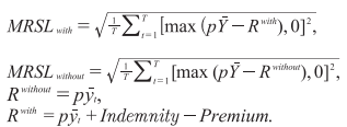
Where p is the price of maize,  is the long-term average of the crop yield and  is the yield. [Poudel et al., 2019] employed the weather derivatives method to price rainfall index insurance and concluded that the average premium rates were 8.8%, thus, reducing the risk exposure of the farmers that purchase the index insurance contract by an average of 26% using the mean root squared loss to compare the risk exposures. J. Kath [Kath et al., 2018] found that the contract including flood cover for sugarcane was inefficient in risk reducing as the contracts with strike price at 70^th and 80^th percentiles as their trigger increased the losses; and the 90^th and 95^th percentiles exhibited no change in the losses. J.K. Poussin and coauthors [Poussin et al., 2015] used the regression models to evaluate the effectiveness of risk reduction and found that useful risk management tools include the household mitigation strategies.

2. Data and methodology

The maize yields and rainfall data used were obtained from AGRITEX and NASA website respectively. For the study, the data ranged from October 2009 to May 2019 for rainfall data and the period from 2010 to 2019 for the maize yields data were used. The Black-Scholes optional pricing framework was used to assess the contract in the study. Normalized yields and seasonal rainfall data for the region were used in the premium estimation process. Regional data were obtained from averaging the district data in the corresponding regions. The MRSL was calculated for the case where there is no insurance and for the case where there is index insurance. The MRSL was calculated using the revenues for both cases.

3. Empirical results and discussion

This section summarises the descriptive statistics (tools, standard deviation, minimum and maximum) of the data used in the research. The descriptive statistics for the sample districts that is used to come up with the regional data are presented in the table 1. According to [Mushore, 2013], the Zimbabwean rainfall season ranges from mid of November to mid of March of the following year. Therefore, the cumulative seasonal rainfall in this study was taken as the cumulative rainfall for the period from the beginning of October to the beginning of May to account for the late planted crops, contradicting with [Mushore et al., 2017] the period ranged from the 1^st of October to the 31^st of March of the next year. The seasonal descriptive statistics for the respective regions for the period 2010-201is summarised below.

The average rainfall received in region I, IIA, IIB, III, IV and V is 701.39 mm, 759.96 mm, 743.45 mm, 660.02 mm,
468.25 mm and 324.95 mm respectively. The average rainfall generally decreases across the regions.

3.1. Analysis of relationship between maize yield
and seasonal rainfall

The relationship between the maize yields and rainfall was examined using different regression models that include linear, log linear and quadratic models. The maize yields data were detrended and normalized to remove the effects of heteroskedasticity and time trends using model 1 and 2. The normalized maize data is presented in the appendix. To test the relationship between the variables the original seasonal data were used in the case of independent variable and normalized maize yields were used in the place of dependent variable. The correlation coefficients R² were compared. The results from the regression models analysis are summarised in the table 2.

The relationship between maize yields and rainfall was modelled better using the quadratic regression model (for all regions) compared to linear regression and nonlinear regression for region I, IIA, IIB, III, IV, V respectively. This is indicated by the highest R² values of 0.01, 0.07, 0.22, 0.03, 0.26 and 0.01 for regions I, IIA, IIB, III, IV and V respectively being obtained from the quadratic regression model; This showed that the maize yields increase with rainfall to a limit point where it starts to decrease with excessive rainfall. Beyond this point the maize yields begin to decrease hence the need for index insurance that will cover both drought and floods. This is similar to the findings of [Mushore et al., 2017], who concluded that the relationship between maize yields and rainfall in Mt Darwin is better modelled by a quadratic regression model with R²= 0.630. These findings are also in contradiction with those of [Poudel et al.,
2019] who found that the crop yields were linearly related to the rainfall data. This is due to the difference in the crop type examined and the sample population.

3.2. Premium Rate estimation

Determination of trigger values. The trigger levels for drought coverage were the lower percentiles i.e. (10^th, 25^th, and 50^th percentiles) whereas the upper percentiles i.e. (60^th, 75^th, and 90^th percentiles) were used as the trigger levels of the floods coverage. Therefore, the trigger values for the contract will be (10^th and 60^th), (25^th and 75^th) and (50^th and 90^th). The percentiles for each region are summarised in table 3.

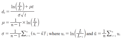
Lognormal test of seasonal rainfall data. When pricing the options using the Black-Scholes framework it is assumed  to follow a lognormal distribution. Hence it is necessary to examine if  follows a lognormal distribution. Q-Q plots for the rainfall data were plotted to indicate that the data follows a lognormal distribution, the plots are presented in the appendix. To prove that the data follow a lognormal distribution, Kolmogorov – Smirnov Test and Shapiro – Wilk Test were carried out using SPSS.

H_o = the ln (seasonal rainfall) follow Normal distribution.

H₁ = the ln (seasonal rainfall) do not follow Normal distribution.

The p-values of the both the Kolmogorov test and Shapiro – Wilk test are both greater than 0.05, therefore we conclude that the natural logarithm of the seasonal rainfall data with maize follows a normal distribution hence the data follow a lognormal distribution, hence we accept H_o. The results of these tests are presented in table 4 below.

Pricing. In this case we consider a contract that pay out indemnity at a rate of 1 in the event of either drought or floods. Therefore:

Pay-out = Pay-out rate x the insured amount of yields x the preagreed value of 1 unit of maize yields.

The contract resembles an exotic combination option, which consists of a cash or nothing put option struck at the lower percentiles and a cash or nothing call option struck at the upper percentiles. Therefore the premiums paid by the insured will be the total of the premiums paid if the farmer were to purchase these options separately (drought and floods insurance separately).

Premiums = Premium of long cash or nothing put option + premium of a long cash or nothing call option.

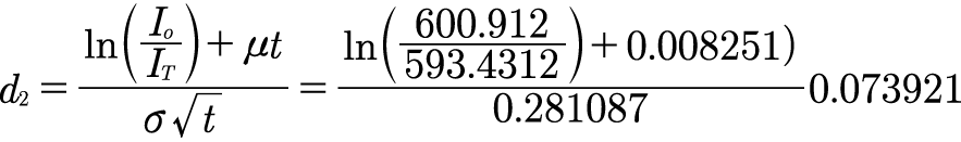
The premiums paid by a farmer from region 3 are calculated as follows:

I₀ = the last entry of the cumulative seasonal rainfall as it is the most recent, in the case of region IIB = 600.912

t = 1

σ = 0.28108

r = 0.05 (assumed)

Price of cash or nothing put option = Payout × e^–rt × N(–d₂)

N(–d₂) = 0.470537

I_T = the 10^th percentile = 593.4312

Payout rate = 1

Premium of put option = 1×e^–0.05 × 0.470537 = 0.447588

Price of cash or nothing call option = Payout × e^–rt × N(d₂)

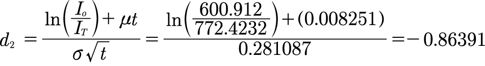
N(d₂) = 0.19382

I_T = the 60^th percentile = 772.4232

Payout rate = 1

Price of cash or nothing call option = Payout × e^–rt × N(d₂) = 1×
× e^–0.05 × 0.19382 = 0.184367

Overall premium = Price of cash or nothing put option + Price of cash or nothing call option = 0.447588 + 0.184367 = 0.631955

There premium rate paid for both drought and floods cover is 0.631955 for a payout rate of 1 in the event of either floods or drought.

Premium price effects of trigger levels

The premium rates for other regions at different trigger levels, i.e. percentiles are summarised in table 5. From this table it can be deduced that for region 3 the premiums grow with an increase in trigger value, hence highlighting the importance of trigger values when pricing the contract. The premium for the drought cover increased by 30.34% when the trigger grew from 493.084 mm (10^th percentile) to 580.734 mm (25^th percentile). When the trigger grew from 693.067 mm (60^th percentile) to 752.37 mm (75^th percentile) the premium rate for the floods scenario cover decreased by 62.98%. The overall premium increased by 20.89%. The percentage changes of premiums as the trigger values increase are summarized in table 6.

We concluded that on average when the trigger value for the drought cover increases, the price of the contract also rises as the probability of rainfall being lower than the trigger value, hence there are higher chances of loss materialization to the insurance company. This conclusion is also similar to that of [Nyawo, 2017] who found out that the price of drought index insurance increases with trigger levels. The cost of floods insurance cover decreases with the increase in the trigger levels of the contract due to poor probability of the payment with lower expectation of costs.

Risk Reduction. To evaluate the effectiveness of the contract the current price of maize was 1171 USD per tonne in May 2019 according to FAO (2019). The study compared the changes in the mean root square loss in the situation of index insurance and visa versa. The MRSL model below was applied, the results of the model are presented in the table 6.

The Mean Root Squared Loss method was applied for all combinations of trigger levels to examine the performance of the index insurance in risk reduction. The results of the evaluation showed the same pattern for all the combinations in the table 6. The analysis of MRSL showed that the contract was efficient in reducing risk for all the trigger levels for all the regions. The greatest risk reduction was experienced. These finding are similar to those of [Poudel et al., 2019] who observed no risk reduction on their study on wheat. They also observed risk reduction on the out-of-sample category for rice. Authors [Kath et al., 2018] also observed no risk reduction for all trigger levels.

4. Conclusions and policy recommendations

The effectiveness of the contract in risk reduction was evaluated by comparing the mean root square loss of the farmer with and without insurance. It was observed that the combination of trigger levels used for the contract was efficient as positive percentage changes of MRSL were observed between the two scenarios for all regions.

The research observed that maize index insurance is viable in Zimbabwe and efficient in risk reduction hence the product is recommended to be used as risk mitigation tool for smallholder farmers. It was found that for the product to be attractive and economically viable the index should be accurately measured and this can be done when the equipment at the meteorological centres is modernized. Hence, there is a need for modernization of the stations. There is a need for IPEC to introduce a regulatory framework to provide standards that will protect the consumer and the provider. These standards will include clear index certification and minimum capital to liability holdings for the providers. The regulator should also update the existing definition of insurance to accommodate index insurance.

The government, IPEC, and Non-Governmental organizations among other stakeholders should consider subsidies to the firms that will pilot the introduction of the index-based insurance product to cushion them from adverse effects of large sunk costs. These costs arise from educating the smallholder farmers, as a majority of them are not fully aware of the formal insurance product existence.